Examples
The examples are organized by material dimensionality. Each case follows the same workflow:
Generate
model.xyzfor GPUMD andbasis.infor pySED.Run GPUMD to create
dump.xyz.Run pySED in compute mode with
plot_SED = 0.Run pySED in plotting mode with
plot_SED = 1.Optionally fit Lorentzian peaks and compare with lattice dynamics.
Each material section links to its example folder and embeds representative output figures from that system, so users can inspect the expected SED result before running the workflow. The advanced notes also embed the Partial SED and LO-TO splitting images discussed in the linked GitHub issues.
1D Systems
Carbon Nanotube
- Purpose
Learn how to set up and analyze SED for a one-dimensional material.
- Folder
Workflow
cd example/CNT/structure
python generate_gpumd_xyz.py

cd ../gpumd_run
gpumd

cd ../SED
pysed input_SED.in
The CNT example uses a 1 x 1 x 160 supercell and the q-path G-A along
the tube axis. After the compute run, set plot_SED = 1 to generate the SED
figure. The example also enables all-q-point Lorentz fitting after the peak
settings are tuned.
Representative result

- Expected outputs
CNT.SED,CNT.Qpts,CNT.THz,CNT-SED.svg, Lorentzian fitting plots, andTOTAL-LORENTZ-Qpoints.Fre_lifetimewhen all-q fitting is enabled.
2D Systems
In-Plane Graphene
- Purpose
Learn how to compute an in-plane SED map for a two-dimensional material and compare the result with lattice dynamics.
- Folder
Workflow
cd example/In_plane_graphene_gpumd/structure
python generate_gpumd_xyz.py

cd ../gpumd_run
gpumd

cd ../SED
pysed input_SED.in
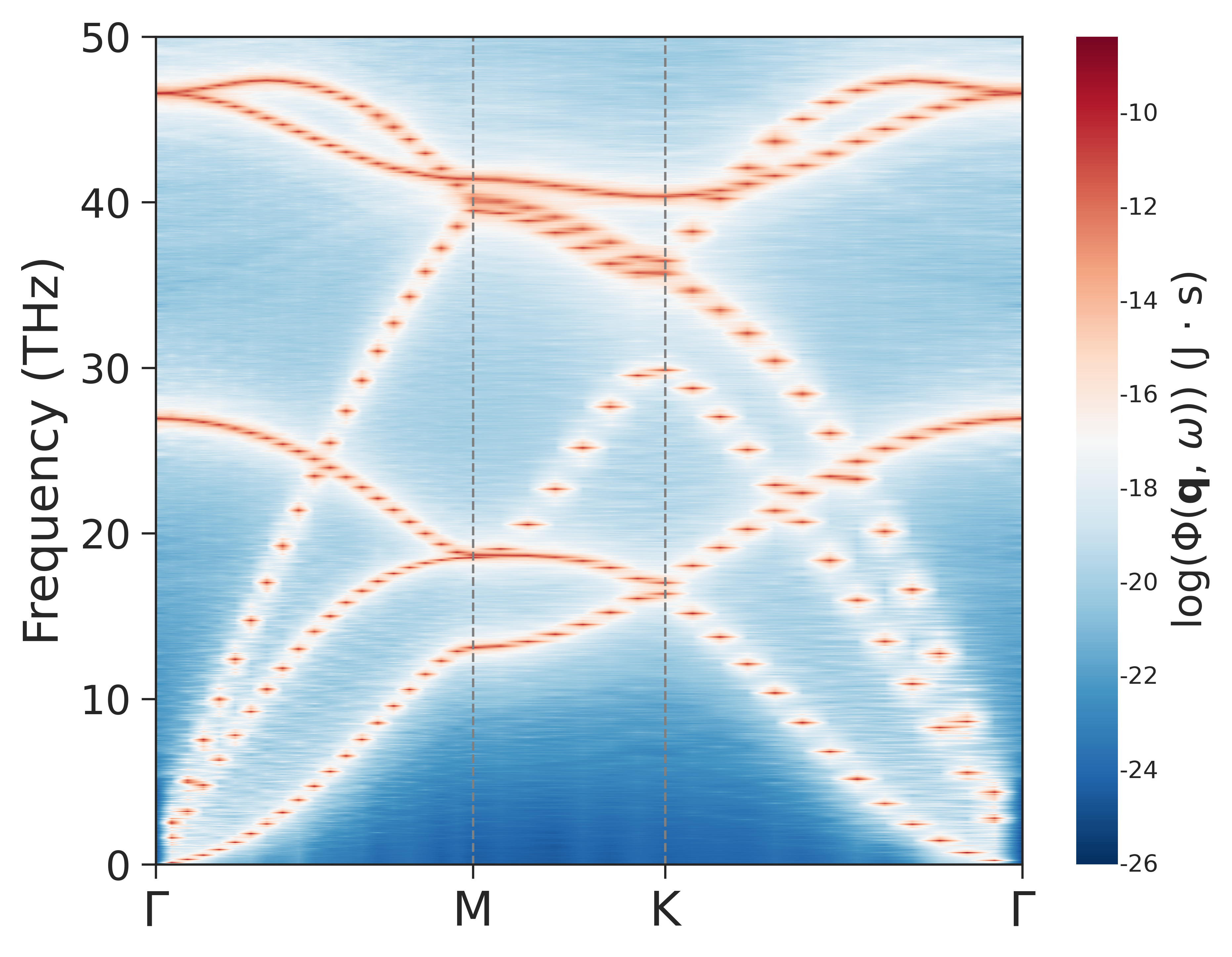
The graphene example uses a 40 x 40 x 1 supercell and the path
G-M-K-G. It uses use_contourf = 1 for a cleaner multi-path plot.
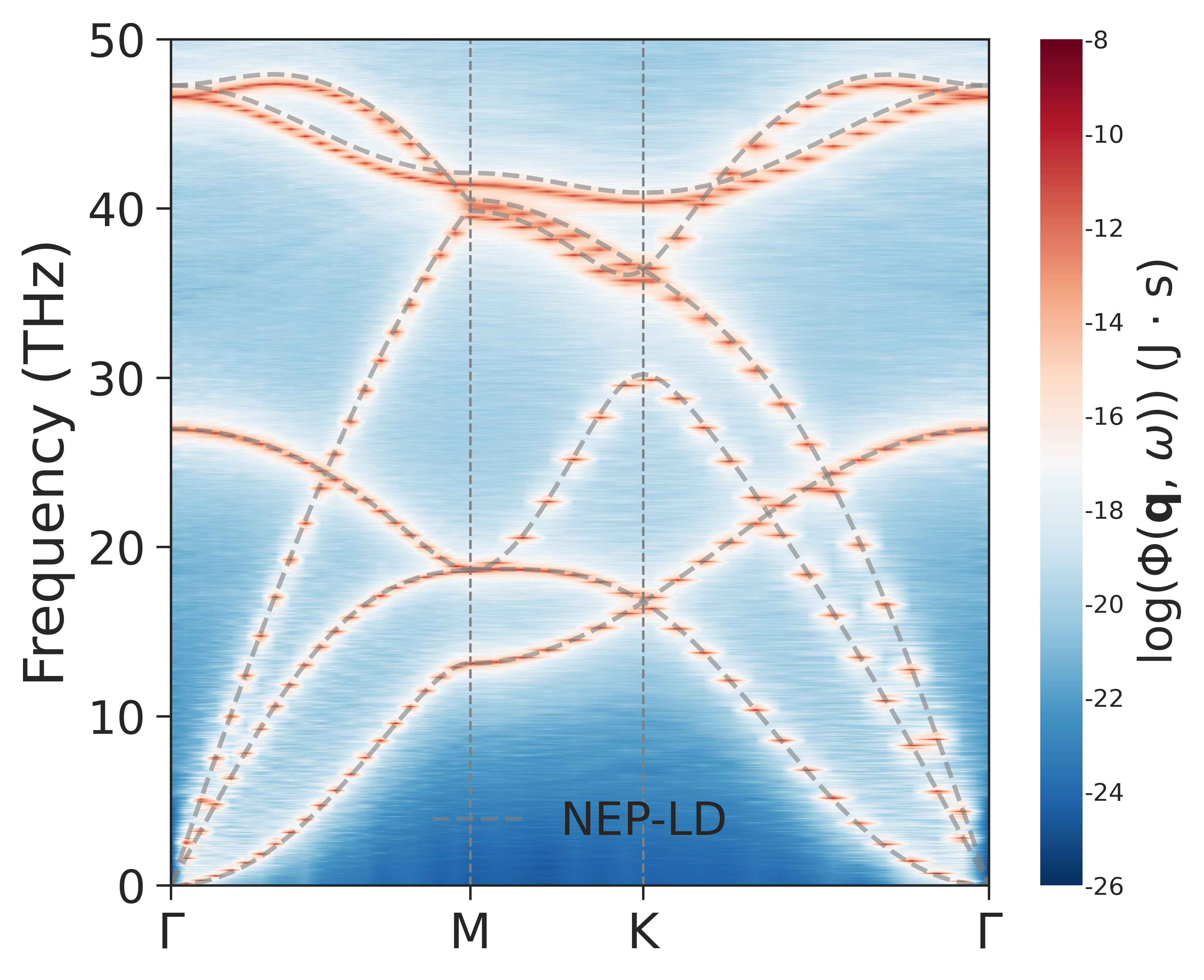
- Lattice-dynamics comparison
The
SED/compare_LDdirectory contains scripts for calculating NEP-driven lattice-dynamics dispersion and overlaying it on the pySED result.
Representative results
Raw pySED SED map:
SED with lattice-dynamics branches:
MoS2 Out-of-Plane Modes
- Purpose
Learn how to analyze low-frequency out-of-plane modes in a layered two-dimensional material.
- Folder
Workflow
cd example/MoS2_gpumd/structure
python generate_lammps_data.py

cd ../gpumd_run
gpumd

cd ../SED
pysed input_SED.in
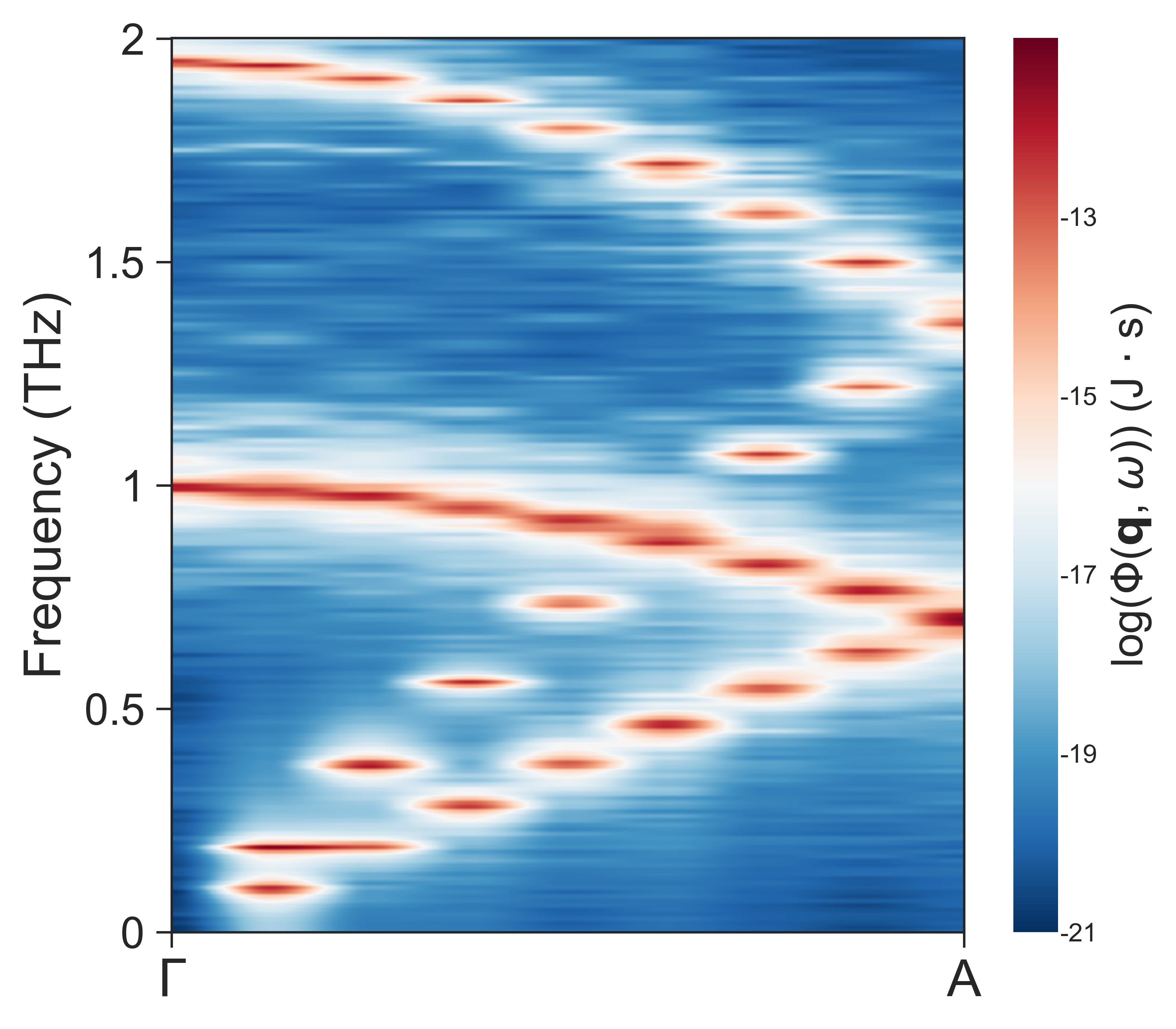
The MoS2 example uses a 12 x 12 x 16 supercell and the q-path
G-A. The low-frequency range is important, so the example uses
plot_cutoff_freq = 2 and a small plot_interval.
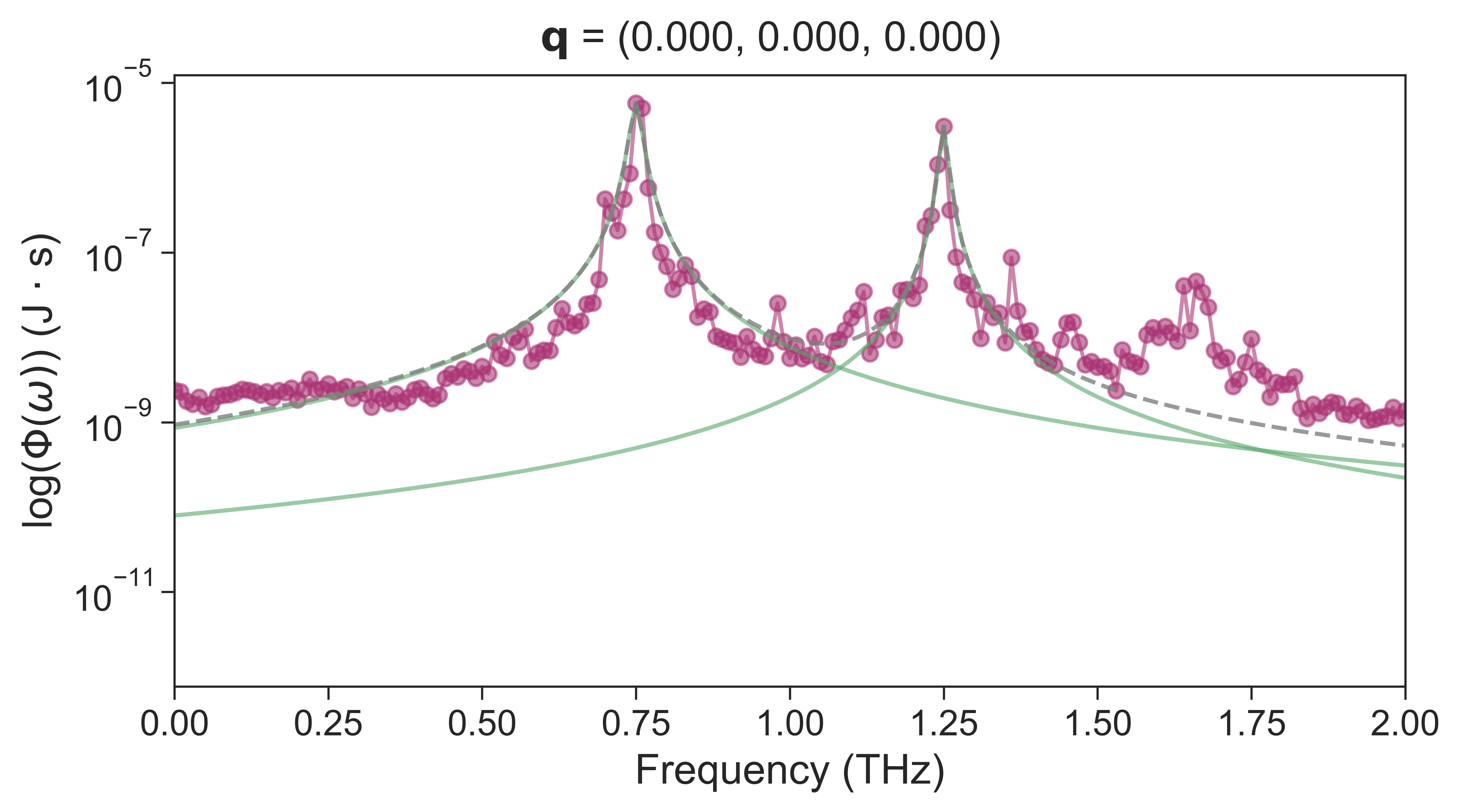
- Fitting
The folder includes Lorentzian fitting results and
TOTAL-LORENTZ-Qpoints.Fre_lifetime. Use the existing files to learn how peak thresholds affect low-frequency lifetime extraction.
Representative results
Low-frequency out-of-plane SED:
Single-q-point Lorentzian fitting example:
3D Systems
Bulk Silicon
- Purpose
Learn how to perform SED analysis for a three-dimensional crystalline material and compare the result with lattice dynamics.
- Folder
Workflow
cd example/Silicon_primitive_gpumd/structure
python generate_lammps_data.py

cd ../gpumd_run
gpumd

cd ../SED
pysed input_SED.in
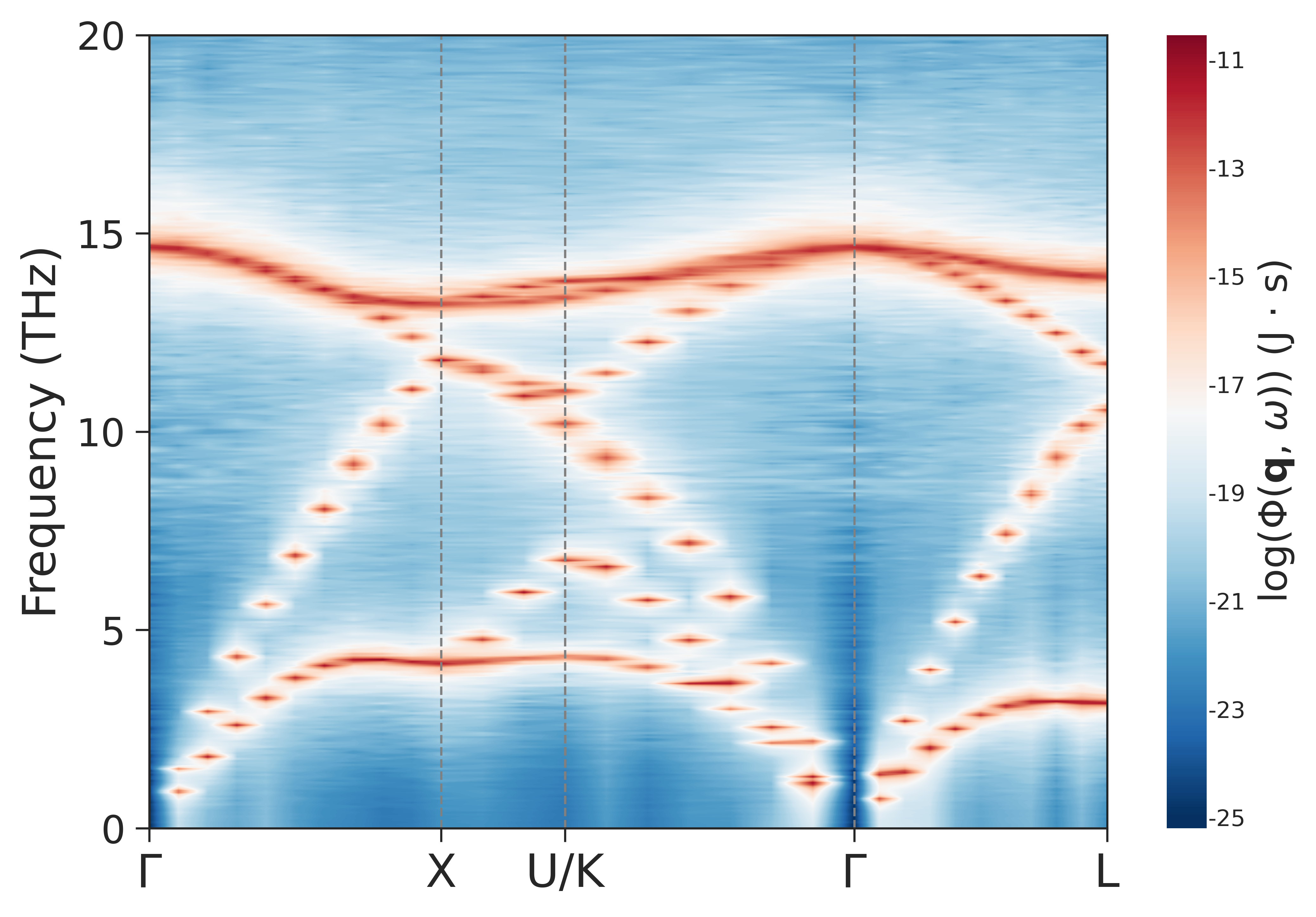
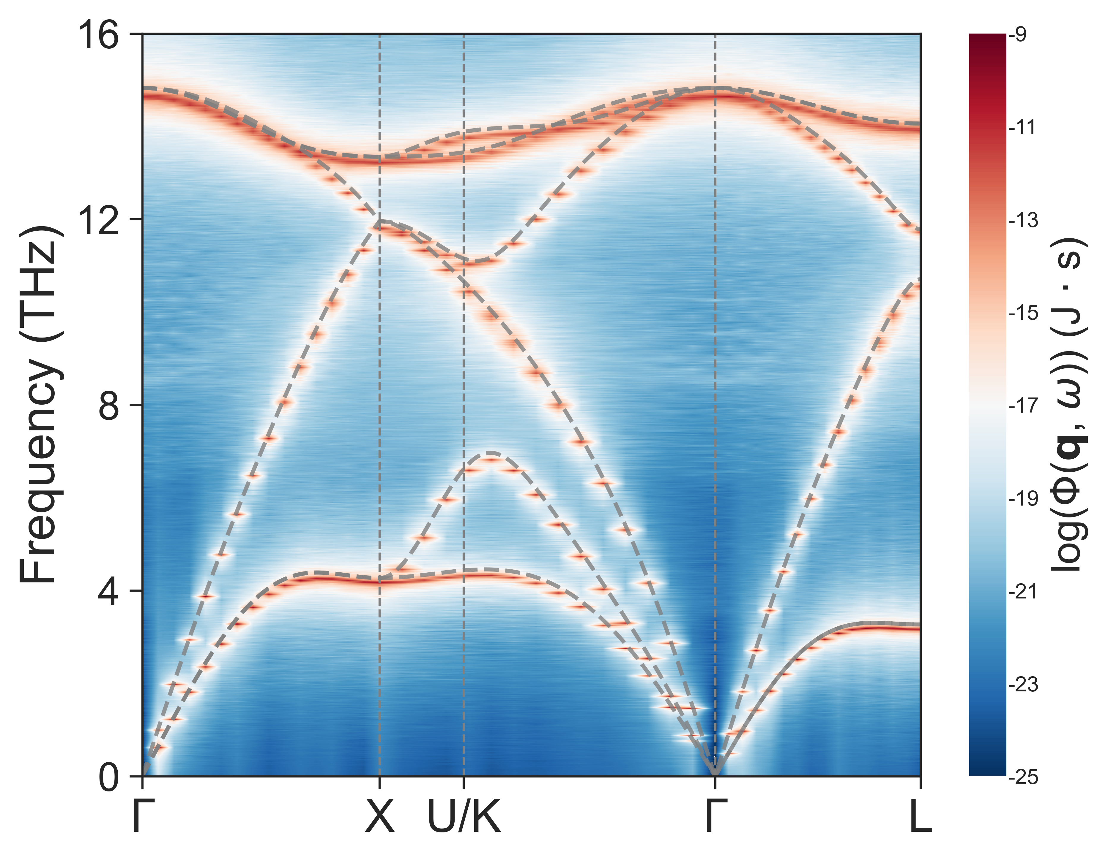
The silicon example uses a 20 x 20 x 20 supercell and the path
G-X-U-K-G-L. It is a good starting point for checking multi-segment q-paths,
prim_unitcell consistency, and phonon dispersion comparison.
- Lattice-dynamics comparison
Use the scripts in
SED/compare_LDto compare pySED output with NEP-driven lattice dynamics.
Representative results
Raw pySED SED map:
SED with lattice-dynamics branches:
Advanced Examples and Notes
Partial SED
Partial SED decomposes the SED intensity by atom type and Cartesian direction. Use it when you want to see which species or vibration direction contributes to particular branches.
In compute mode:
plot_SED = 0
output_partial = 1
In plot mode:
plot_SED = 1
plot_partial_SED = 3
plot_partial_SED = 3 x
plot_partial_SED = 3 plots the summed x+y+z contribution for atom type
3. plot_partial_SED = 3 x plots only the x-direction contribution for atom
type 3.
The following SrTiO3 cubic examples from issue #39 show atom-type and direction-resolved partial SED output for Sr atoms:
Sr atoms, x direction:
Sr atoms, y direction:
Sr atoms, z direction:
Partial SED is not local spatial-bin SED. pySED requires a supercell-to- primitive-cell mapping for reciprocal-space q-points, so arbitrary local SED for selected spatial bins is not currently supported.
LO-TO Splitting
For polar materials, pySED can show LO-TO splitting only when the MD trajectory already contains the corresponding long-range Coulomb physics. A trajectory from a model without the relevant long-range electrostatics will not gain LO-TO splitting during pySED post-processing.
When comparing with lattice dynamics, use NAC in the reference calculation if the material requires it. Differences between finite-temperature SED and lattice dynamics can also come from anharmonicity or from the level of theory used for the potential, Born charges, and dielectric constants.
The following BaTiO3 examples from issue #31 illustrate the trajectory-dependence of the LO-TO splitting:
NEP trajectory compared with NEP-driven lattice dynamics without applying a non-analytical correction:
qNEP trajectory compared with qNEP lattice dynamics including the non-analytical correction. The SED captures the LO-TO splitting already present in the trajectory:
More Examples
Additional examples and older LAMMPS workflows are available in the pySED example library.